The random vibration workflow

A controller run in, a compliance report out. A random test is judged against a band: the specification says what the control PSD must be, warning and abort lines say how far it may stray, and the report's job is to show where the run sat inside that band, channel by channel.

The walkthrough is the demonstration plate's own random test — eight control channels against four shakers, controlled to a shaped specification by a real Rattlesnake run — photographed at every step. The run ships with the repository (testdata/plate/random.nc4), so every step can be followed exactly.

Step	In the app	In a script
Import the run	drag the controller's .nc4 onto the window	project = visualdynamics.random_vibration_run(path)
Say what it is for	(the run says — the type switches itself)	project.project_type == 'Random Vibration'
Control PSDs	Compute PSDs in the averaging view	project.compute_psds('Time History')
The octave-band view	Octave Bands on the PSD's bar	project.compute_octave('Time History PSDs')
Multiple coherence	Multiple Coherence in the averaging view	project.compute_multiple_coherence('Time History')
Compare against the spec	select PSD and specification together	plot_comparison(psds, spec)
Geometry and photos	drag them in, link them	project.add(...), project.link(...)
Report	Generate Report on the bar, the project row selected	project.generate_report('random')
Export	Export HTML…	project.export_report(name, path)
Save	Save Project As…	project.save('random.vdyn')

In the app, step by step

1. Import the run

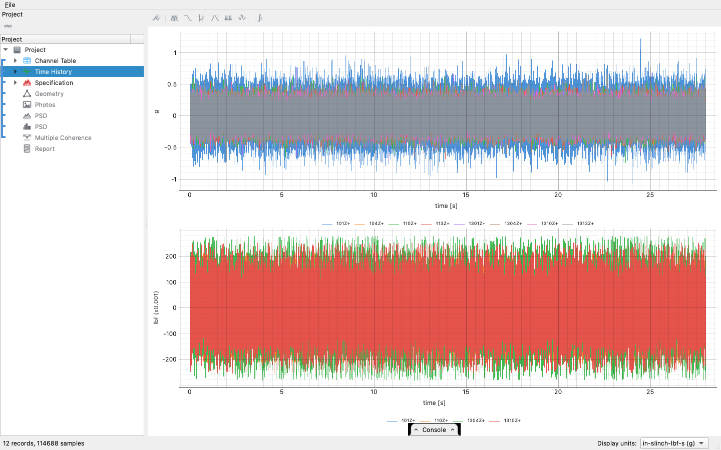
Drag the controller's save onto the window. A Rattlesnake random run brings the control time histories, the specification with its warning and abort lines, and the channel table in one file — and says which environment drove it, so the project type switches to Random Vibration by itself. The tree's gray slots then say what a finished report still needs.

A run too long to hold whole asks first: the import window shows one channel's envelope over the whole run, and the stretch to import is chosen on it — dragged, typed as a start and a stop, or typed as the Last so many seconds of the run, which is the usual answer for a long run whose end is the stretch at level. A run shorter than that is imported whole.

2. Compute the control PSDs

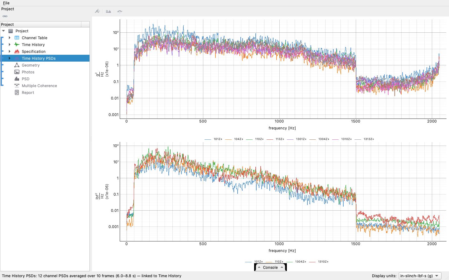
Compute PSDs in the time history's averaging view averages over the run's own frame length, overlap and window — the controller's, read from the file, not guessed — with the start and the count worked out from the record itself: where the run is at level and how many frames that stretch holds, the same answer the view's Detect button gives. The view shows exactly those frames before the button is pressed.

3. Band onto sixth octaves

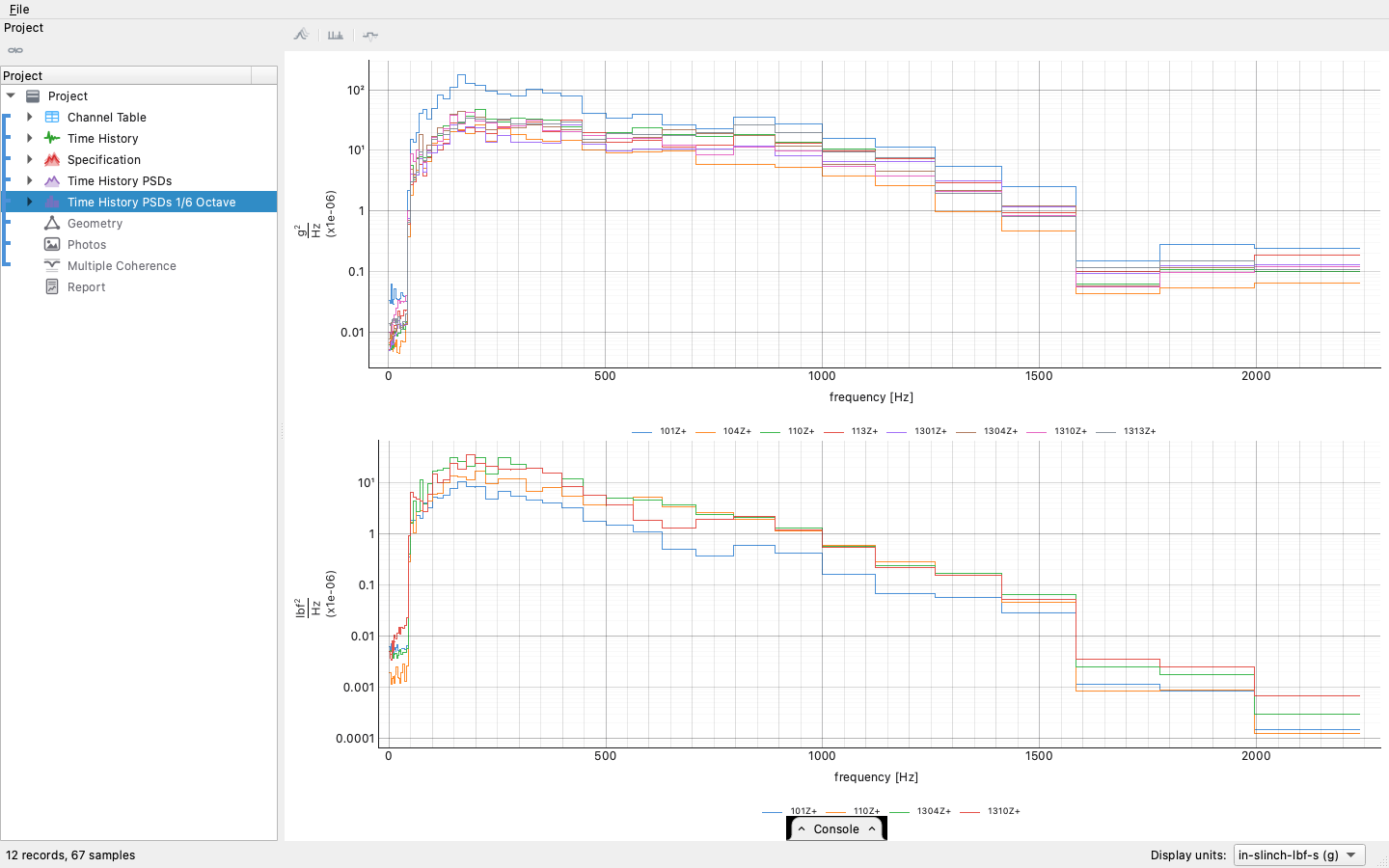
The octave-band PSD is a standing deliverable of a random report, not an option, and so is the specification on the same bands. Octave Bands on the PSD's bar previews the banded steps over the narrowband as the spacing is set (a sixth is the usual answer) and the panel's own button bands conserving area — the octave PSD is still a PSD, drawn as bars because its bandwidth says so. The same button on the specification bands the requirement and its warning and abort limits together, and the report's octave section reads the banded measurement against that banded requirement rather than against the breakpoint curve.

The report opens on a pass/fail box under its title: PASS in green or FAIL in red, read off the octave-band comparison, with the two readings it was decided on beside it — the share of control channels that had more than a tenth of their band outside the abort limits, failing at a fifth of them, and the share more than 3 dB off in RMS, failing at a tenth. Someone opening the report knows whether the environment passed before reading a word. The octave-band figures read on a log frequency axis, the narrowband ones on a linear one.

The report draws the measured time histories flat, two dozen channels to a figure and as many figures as the run has channels, each figure an envelope of its channels on one shared time axis with the averaged frames marked. A 144-channel run at 16 kHz was a 200 MB report when those figures were the stage; they are a few megabytes now, and every number on the page keeps seven significant digits, which draws a figure to a part in ten million.

4. Multiple coherence

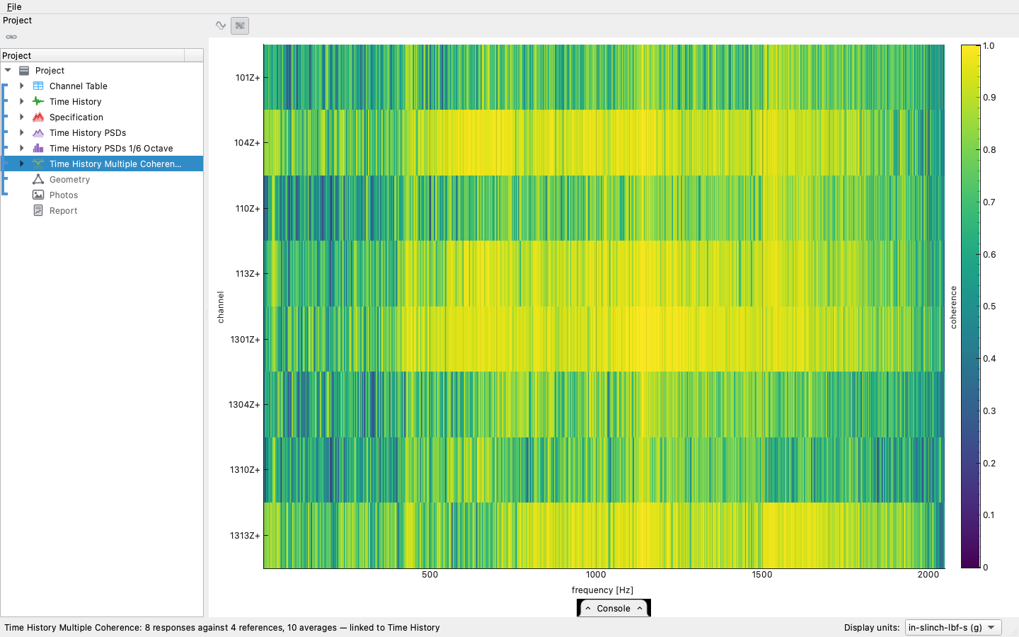
How much of each response the drives account for — Multiple Coherence, beside the PSDs in the averaging view, so it reads the same frames. This is the figure that later separates "the article exceeded" from "the cable did" — a channel the drives explain (coherence near one) exceeded because the article did.

5. Compare against the specification

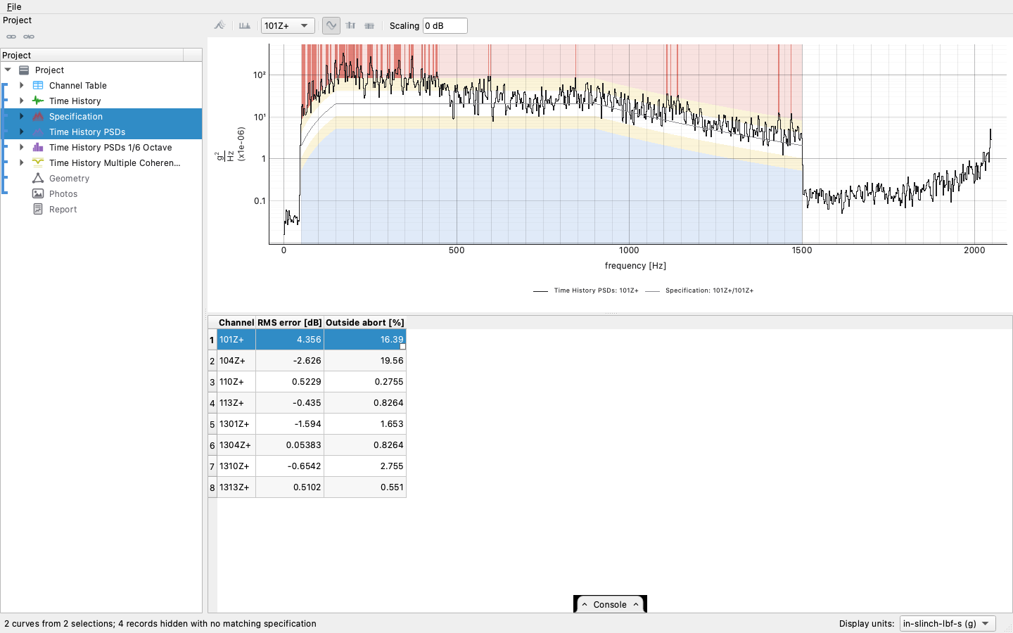
Select the control PSDs and the specification together. One channel draws at a time — the drop-down reaches the rest — with the tolerance zones shaded and every line that went outside the abort band striped red or blue for which way it went. The table below the plot accounts for every channel at once; the plot shows the ones you pick in it. How a line or a band is judged in or out — an area against an area over each cell, whatever form the two objects take — is its own page.

Two things to notice in the bar above the plot. The Scaling field is the comparison's dB offset — detected from the data to the nearest 3 dB, the ladder runs are commanded on, for runs captured below the 0 dB requirement; this run was at full level, so it reads 0. And the status bar notes the records that had no specification to answer to: the drive force PSDs share DOF names with control channels, and the comparison filters them out rather than judging newtons against an acceleration band.

6. Geometry, photos, report

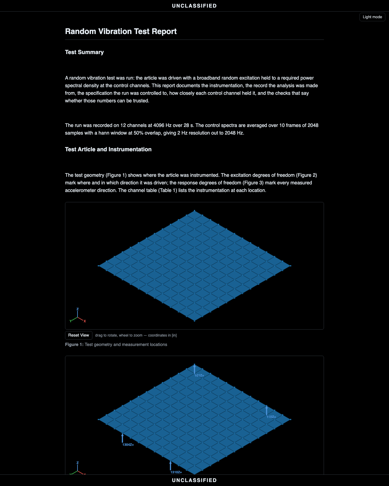
Drag the article's geometry in and declare its units; drop the setup photographs beside it; link them into the group. Then the project's row's Generate Report builds the random report — the measured data, the specification comparison read three ways (spectra, RMS error bars, lines-out bars), the coherence beside the compliance so the reader can ask why a channel exceeded. The specification and the comparison are one figure per control channel — no drop-down anywhere in the report — narrowband and again on octave bands against the banded specification, each comparison opening on the specification's own frequency band with the measurement beyond it a zoom away; a banded specification is drawn on its own bands, steps against steps. Above four control channels the figures become a grid instead: a row per node, a column per direction — the global axes when the linked geometry can place the channels, with how far off its axis a channel sits noted in its cell, the DOF's own letter when it cannot — and each cell is the figure that channel alone would have had. The channel table keeps every row on one line, however long its comments. A section whose objects the project does not hold — the specification sections of a run imported without one, say — is left out of the report rather than standing as a heading over nothing. Export → HTML… writes one self-contained file.

The same run, headless

And the script never has to be reconstructed by hand: the console tab along the bottom of the window writes it live as you click — every act of the session as the line that replays it. Expand it, copy the stretch you want, and it runs as-is.

The whole thing is one call when the defaults are right:

import visualdynamics

visualdynamics.random_vibration_report('random.nc4', 'report.html')

…and still one call when the report needs the rest of what the tree asks for. The geometry comes in with its length unit declared when the file does not carry one, the photographs from a folder (or a list of files, in the order they should appear), and a run too long to hold is read from its last so many seconds — a shorter run is taken whole:

visualdynamics.random_vibration_report(
    'random.nc4', 'report.html',
    geometry='article.stp', length_unit='mm',
    photos='setup_photos/',
    last=100.0)

…and the same call written out when the project should live on. It is condensed from examples/random_workflow.py, which the test suite executes; the step numbers match the walkthrough.

import visualdynamics
from visualdynamics.plot import plot_bars, plot_coherence_map, plot_comparison

# 1-4. import and work up: PSDs over the run's own frames, the
# sixth-octave banding, the coherence — one verb does the sequence
project = visualdynamics.random_vibration_run('random.nc4')
assert project.project_type == 'Random Vibration'

history = project.time_history
spec, octave_spec = project.specifications   # the requirement, and it on bands
psds, octave = project.psds                  # the specifications are not among them

# 5. the comparison, drawn headless — bands against bands
plot_comparison(psds, spec, path='control.png', show=False)
plot_comparison(octave, octave_spec, path='control_octave.png', show=False)
plot_bars(psds, spec, 'error', path='error.png', show=False)
plot_bars(psds, spec, 'lines', path='lines.png', show=False)
plot_coherence_map(project.coherence, path='coherence.png', show=False)

# 6. geometry, photos, report
project.add('Geometry', visualdynamics.import_file('geometry.npz'))
project.geometry.define_units('m')
project.link(*project.names)
project.set_basis(*project.names)
project.generate_report('random')
project.export_report(project.report, 'random_report.html')
project.save('random.vdyn')

Where judgment lives

• Whether an exceedance is the article or the instrumentation. The multiple coherence map answers it: a channel whose response the drives explain exceeded because the article did; a channel low on coherence may be a mounting or a cable. The report puts the map beside the compliance bars for exactly this reading.
• Whether the comparison scale is right. A run captured below the requirement is compared scaled up to the 0 dB specification — standard practice — and the scale is detected only when the data supports it: every channel at or above a corroborated offset. Type a number in the Scaling field to hold it (0 holds it unscaled), clear the field to detect again. The data itself is never changed.
• What the run was allowed to do. The warning and abort lines come from the specification; whether a brush against the warning line matters is the test engineer's sentence to write in the conclusions.